Building a Multiple Linear Regression Model

Previously, we have seen situations where an outcome (the dependent variable) is based on a single input variable (independent variable). Sadly, real life is rarely as simple. Most outcomes in real situations are affected by multiple input variables. To understand such relationships, we use models that use more than one input (independent variables) to linearly model a single output (dependent variable).

A multiple linear regression model is a linear equation that has the general form: y = b₁x₁ + b₂x₂ + … + c where y is the dependent variable, x₁, x₂… are the independent variable, and c is the (estimated) intercept.

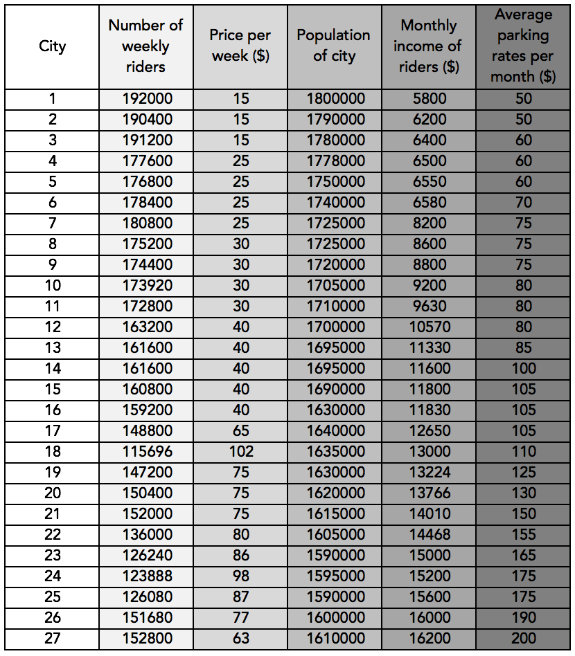
Let us try with a dataset. I downloaded the following data from here:

You can download the formatted data as above, from here.

In the above data, the ‘Number of weekly riders’ is a dependent variable that depends on the ‘Price per week ($)’, ‘Population of city’, ‘Monthly income of riders ($)’, ‘Average parking rates per month ($)’.

Let us assign the variables:

• Price per week ($) – x₁
• Population of city – x₂
• Monthly income of riders ($) – x₃
• Average parking rates per month ($)- x₄
• Number of weekly riders – y

The linear model would be of the form: y = ax₁ + bx₂ + cx₃ + dx₄ + e where a, b, c, d are the respective coefficients and e is the intercept.

There are a two different ways to create the linear model on Microsoft Excel. In this article, we will take a look at the Regression function included in the Data Analysis ToolPak. Please look here to see details on how to enable the Data Analysis ToolPak on your computer.

After the Data Analysis ToolPak has been enabled, you will be able to see it on the Ribbon, under the Data tab:

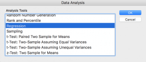
Click Data Analysis to open the Data Analysis ToolPak, and select Regression from the Analysis tools that are displayed.

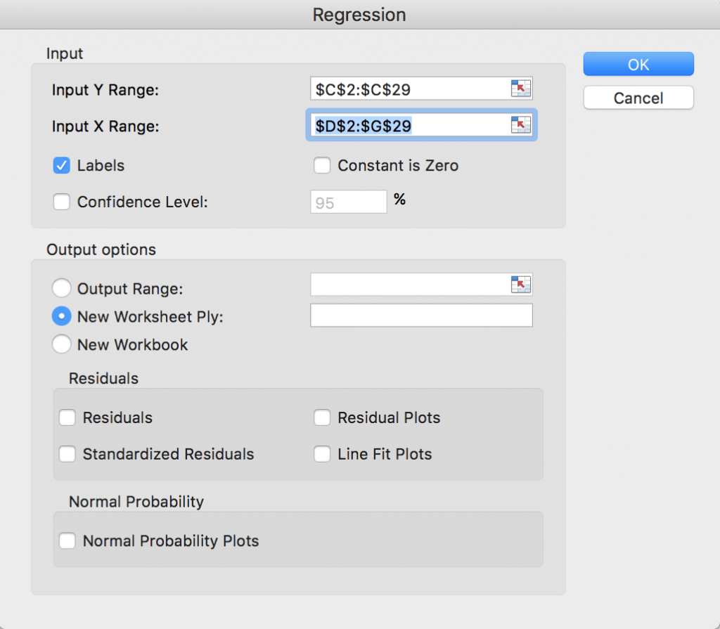
Select the data ranges in the options:

The output looks like this:

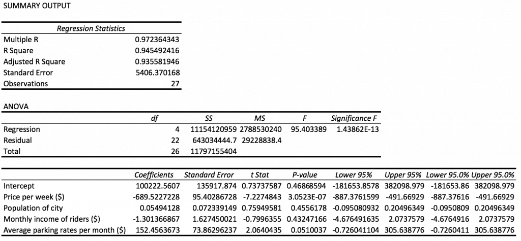
Right on top are the Regression Statistics. Here we are interested in the following measures:

• Multiple R, which is the coefficient of linear correlation
• Adjusted R Square, which is the R Square (coefficient of determination) adjusted for more than one independent variable

We are also interested in the coefficients at the bottom. We are most interested in the Coefficients column. The Lower 95% and Upper 95% columns give the lower and upper limits for the coefficients. We see that the following are the coefficients:

• Price per week ($): -689.5227
• Population of city: 0.0549
• Monthly income of riders ($): -1.3014
• Average parking rates per month ($): 152.4563
• Intercept: 100222.5607

The linear equation is:

We can also build the linear model using the LINEST function (array formula) in Excel. The syntax of the LINEST function is =LINEST(known y’s, known x’s, constant, stats) where the constant can be 0 or FALSE (for a model with no intercept), or 1 or TRUE (for a model with intercept). The model would be displayed on consecutive cells along a row, with the last coefficient coming in on the first cell, and the intercept on the last cell.

In the LINEST function, the stats argument can also be 0 or FALSE (to not display additional regression statistics, and 1 or TRUE to display additional regression statistics. If the additional regression statistics are shown, the second row gives the standard error associated with each coefficient (that is displayed on the row above it). The first value in the third row gives the R squared (coefficient of determination).

To learn more about how to enter an array formula, you can read the Excel support pages here (under ‘Create an array formula that calculates multiple results).

The following are the values that can be returned by LINEST:

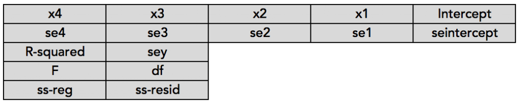
In the above figure:

• x4, x3, x2..: Coefficients
• se4, se3, se2…: Standard errors of the coefficients
• R-squared: Coefficient of determination
• sey: Standard error of y
• F: F-statistic
• df: Degrees of freedom
• ss-reg: Sum of squares of the regression model
• ss-resid: Sum of squares of the residuals

In our dataset, we have four coefficients (x₁ – x₄) and the intercept, making it a total of five values. Therefore, we select five consecutive rows and enter the following as an array formula:

Notice the curly brackets around the function on the formula bar – those denote that it is an array function. The curly brackets are not to be typed directly, they appear when an array formula is entered. The result of the above array formula is:

It would be helpful to clean the results up a little bit. Let us label the values and look at the model. We know that the coefficients are shown in the reverse order, and the intercept is shown at the end:

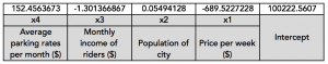
Let us look at the results with the additional regression statistics displayed:

Either of the above methods may be used to build the multiple regression model. In fact, both the above methods would work for univariate regression as well – what we did using the regression trendline earlier.

For multiple regression, using the Data Analysis ToolPak gives us a little more helpful result because it provides the adjusted R-square. The LINEST function gives the R-square value that is not adjusted for the number of terms in the multiple regression model.