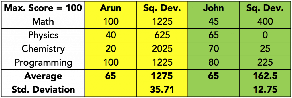
We have already seen how it is easier to describe data using a single measure of central tendency, such as, average. Now, take a look at the following data:
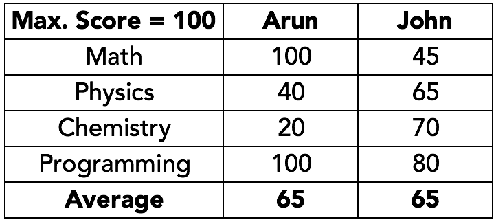
The average score for both students is equal. However, John is consistent at everything, while Arun is brilliant at math and programming, but terrible at chemistry. Clearly, it is difficult to judge the performance of the two students on the basis of their average scores alone. We need some additional measure to reveal the entire story.
Measures of Spread
Since the mean can be affected by extreme values, it is helpful to interpret the mean along with an idea of just how extreme are the values in the dataset. The measures of spread tell us how extreme the values in the dataset are. There are four measures of spread, and we’ll talk about each one of them.
Range
The simplest measure of spread in data is the range. It is the difference between the maximum value and the minimum value within the data set. In the above data containing the scores of two students, range for Arun = 100-20 = 80; range for John = 80-45 = 35. Though the average scores are same for both, John is more consistent because he has a smaller range of scores.
Variance
Dispersion, or spread of data, is measured in terms of how far the data differs from the mean. In other words, if mean is the centre of the data, if we get an idea about how far the individual data points deviate from the mean, we would have an idea about the spread. Therefore, a simple measure of dispersion could be an average of the differences about the mean.
However, this average would have a problem. The actual data points could lie on either side of the mean, and thus, the deviations could be either positive or negative. Now, if we were to compute the average of these deviations, the negatives and positives would cancel out, and the average would be very low, or even zero.
Take a look at the table below; the deviations are calculated as Value minus Mean, and the average of the deviations is calculated:
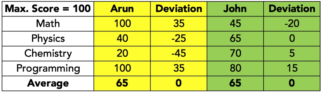
Does this mean that there are no deviations in the data? Clearly, that is untrue.
We need to manipulate the negative values in some way, so as to get rid of the negative sign. This is usually done by squaring the values before computing the average of the squared deviations. The resulting average value is called the variance. In the table below, the deviations have been squared, and then averaged:
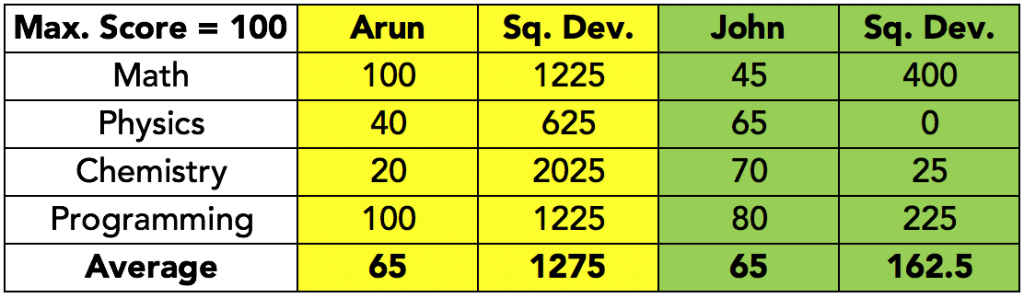
This time, the numbers are more in line with what we would expect – Arun’s scores have a higher deviation, compared to John’s scores.
However, in doing this, while the earlier problem of numbers cancelling out is solved, a new problem emerges – what does the 1275 for Arun really mean? Is it indicative of some squared scores? Now, scores are understandable, but what are squared scores? Values with unit dimensions are meaningless when squared.
Standard Deviation
The meaning is restored to variance, by computing the square root of the variance, thus returning it to the original unit.
The values of the standard deviation do not suffer from the problems of logical explanation like variance, and yet are meaningfully able to convey the magnitude of the deviations. These advantages have made standard deviations the standard measure of deviation calculation in the world of statistics.
Measures using Absolute Deviations
If we are squaring the deviations while computing the variance only to get rid of the squares, we could achieve the same purpose by computing the absolute values of the deviations as well. By computing this way, a few similar measures are possible:
- Mean/Average Absolute Deviation (MAD/AAD) – This is the average of the absolute deviations around the mean.
- Median Absolute Deviation – This is the median of the absolute deviations around the mean.
- Average Deviations – These are the average deviations that are calculated either around mean, or around median.
Inter-Quartile Range (IQR)
When an ordered data set is divided into four parts, the boundaries are called quartiles. If the same data is divided into 100 parts, each part is called a percentile.
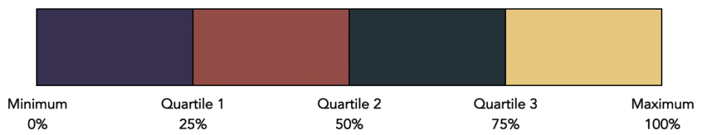
The interquartile range (IQR) is the difference between the Quartile 3 boundary value and the Quartile 1 boundary value. Therefore, the IQR describes the 50% of the data in the middle of the complete set. In terms of percentiles, the IQR is the difference between the 75th percentile and the 25th percentile, which again describes the 50% values in the middle.
The advantage of inter-quartile range is that it considers the middle 50% values and ignores the ones at either extreme. This way, outliers are excluded, unlike in the range calculation the gets impacted by outliers. You can read more about quartiles here.
Computing the measures of dispersion
Now that we have understood the various measures of dispersion, in the next post, we shall look at how we could compute these measures in Microsoft Excel.